Fiscal inflation and interest rates

Economics is about solving lots of little puzzles. At a July 4th party, a super smart friend -- not a macroeconomist -- posed a puzzle I should have understood long ago, prompting me to understand my own models a little better. 

How do we get inflation from the big fiscal stimulus of 2020-2021, he asked? Well, I answer, people get a lot of government debt and money, which they don't think will be paid back via higher future taxes or lower future spending. They know inflation or default will happen sooner or later, so they try to get rid of the debt now while they can rather than save it. But all we can do collectively is to try to buy things, sending up the price level, until the debt is devalued to what we expect the government can and will pay. 

OK, asked my friend, but that should send interest rates up, bond prices down, no? And interest rates stayed low throughout, until the Fed started raising them. I mumbled some excuse about interest rates never being very good at forecasting inflation, or something about risk premiums, but that's clearly unsatisfactory. 

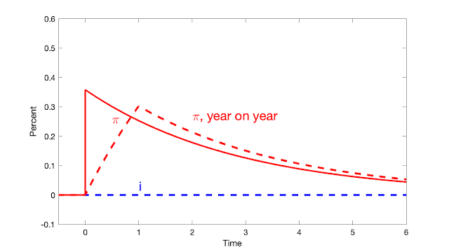
Of course, the answer is that interest rates do not need to move. The Fed controls the nominal interest rate. If the Fed keeps the short term nominal interest rate constant, then nominal yields of all bonds stay the same, while fiscal inflation washes away the value of debt. I should have remembered my own central graph: 

This is the response of the standard sticky price model to a fiscal shock -- a 1% deficit that is not repaid by future surpluses -- while the Fed keeps interest rates constant. The solid line is instantaneous inflation, while the dashed line gives inflation measured as percent change from a year ago, which is the common way to measure it in the data. 

There you have it: The fiscal shock causes inflation, but since the nominal interest rate is fixed by the Fed, it goes nowhere, and long term bonds (in this linear model with the expectations hypothesis) go nowhere too. 

OK for the result, but how does it work? What about the intuition, that seeing inflation coming we should see higher interest rates? Let's dig deeper. 

Start with the simplest model, one-period debt and flexible prices. Now the model comes down to, nominal debt / price level = present value of surpluses, \[\frac{B_{t-1}}{P_t} = E_t \sum_{j=0}^\infty \beta^j s_{t+j}.\] (If you don't like equations, just read the words. They will do.) With a decline in the present value of surpluses, the value of debt coming due today (top left) can't change, so the price level must rise. The price of debt coming due is fixed at 1, so its relative price can't fall and its interest rate can't rise. Or, this model describes a price level jump. We get bad fiscal news, people try to spend their bonds, the price level jumps unexpectedly up, (\(P_t\) jumps up relative to \(E_{t-1}P_t\), but there is no further inflation, no rise in expected inflation so the interest rate \(i_t = r+ E_t \pi_{t+1}\) doesn't change. 

Ok, fine, you say, but that's one period, overnight debt, reserves at the Fed only. What about long term bonds? When we try to sell them, their prices can go down and interest rates go up, no? No, because if the Fed holds the nominal interest rate constant, their nominal prices don't change. With long term bonds, the basic equation becomes market value of nominal debt / price level = expected value of surpluses, \[\frac{\sum_{j=0}^\infty Q_t^{(j)} B_{t-1}^{(j)}}{P_t} = E_t \sum_{j=0}^\infty \beta^j s_{t+j}.\] Here, \(Q_t^{(j)}\) is the price of \(j\) period debt at time \(t\), and \(B_{t-1}^{(j)}\) is the face value of debt at the beginning of time \(t\) that matures in time \(t+j\). (\(Q_t^{(j)}=1/[1+y^{(j)}_t)]^j\) where \(y^{(j)}_t\) is the yield on \(j\) period debt; when the price goes down the yield or long-term interest rate goes up. )

So, my smart friend notices, when the present value of surpluses declines, we could see nominal bond prices \(Q\) on top fall rather than the price level \(P\) on the bottom rise.  But we don't, because again, the Fed in this conceptual exercise keeps the nominal interest rate fixed, and so long term bond prices don't fall. If the \(Q\) don't fall, the \(P\) must rise. 

The one-period price level jump is not realistic, and the above graph plots what happens with sticky prices. (This is the standard continuous time new-Keynesian model.) The intuition is the same, but drawn out. The sum of future surpluses has fallen. People try to sell bonds, but with a constant interest rate the nominal price of long term bonds cannot fall. So, they try to sell bonds of all maturities, pushing up the price of goods and services. With sticky prices, this takes time; the price level slowly rises as inflation exceeds the nominal interest rate. A drawn out period of low real interest rates slowly saps the value of bondholder's wealth. In present value terms, the decline in surpluses is initially matched by a low real discount rate. Yes, there is expected inflation. Yes, long-term bondholders would like to escape it. But there is no escape: real rates of return are low on all bonds, short-term and long term. 

So, dear friend, we really can have a period of fiscal inflation, with no change in nominal interest rates. Note also that the inflation eventually goes away, so long as there are no more fiscal shocks, even without the Fed raising rates. That too seems a bit like our reality. This has all been in my own papers for 20 years. It's interesting how hard it can be to apply one's own models right on the spot. Maybe it was the great drinks and ribs. 

The Fed and the Phillips curve

I just finished a new draft of "Expectations and the neutrality of interest rates," which includes some ruminations on inflation that may be of interest to blog readers. 

A central point of the paper is to ask whether and how higher interest rates lower inflation, without a change in fiscal policy. That's intellectually interesting, answering what the Fed can do on its own. It's also a relevant policy question. If the Fed raises rates, that raises interest costs on the debt. What if Congress refuses to tighten to pay those higher interest costs? Well, to avoid a transversality condition violation (debt that grows forever) we get more inflation, to devalue outstanding debt. That's a hard nut to avoid.  

But my point today is some intuition questions that come along the way. An implicit point: The math of today's macro is actually pretty easy. Telling the story behind the math, interpreting the math, making it useful for policy, is much harder. 

1. The Phillips curve

The Phillips curve is central to how the Fed and most policy analysts think about inflation. In words, inflation is related to expected future inflation and by some measure if economic tightness, factor \(x\). In equations, \[ \pi_t = E_t \pi_{t+1} + \kappa x_t.\] Here \(x_t\) represents the output gap (how much output is above or below potential output), measures of labor market tightness like unemployment (with a negative sign), or labor costs. (Fed Governor Chris Waller has a great speech on the Phillips curve, with a nice short clear explanation. There are lots of academic explanations of course, but this is how a sharp sitting member of the FOMC thinks, which is what we want to understand. BTW, Waller gave an even better speech on climate and the Fed. Go Chris!)  

So how does the Fed change inflation? In most analysis, the Fed raises interest rates; higher interest rates cool down the economy lowering factor x; that pushes inflation down. But does the equation really say that? 

This intuition thinks of the Phillips curve as a causal relation, from right to left. Lower \(x\) causes lower inflation. That's not so obvious. In one story, the Phillips curve represents how firms set prices, given their expectation of other's prices and costs. But in another story, aggregate demand raises prices, and that causes firms to hire more (Chris Waller emphasized these stories). 

This reading may help to digest an otherwise puzzling question: Why are the Fed and its watchers so obsessed with labor markets? This inflation certainly didn't start in labor markets, so why put so much weight on causing a bit of labor market slack? Well, if you read the Phillips curve from right to left, that looks like the one lever you have. Still, since inflation clearly came from left to right, we still should put more emphasis in curing it that way. 

2. Adjustment to equilibrium vs. equilibrium dynamics. 

But does the story work? Lower \(x_t\) lowers inflation \(\pi_t\) relative to expected future inflation \(E_t \pi_{t+1}\). Thus, it describes inflation that is rising over time.  This does not seem at all what the intuition wants. 

So how do we get to the intuition that lower \(x_t\) leads to inflation got goes down over time?  (This is on p. 16 of the paper by the way.) An obvious answer is adaptive expectations: \(E_t \pi_{t+1} = \pi_{t-1}\).  Then lower \(x_t\) does mean inflation today lower than it was in the past. But the Fed and most commenters really don't want to go there. Expectations may not be "rational," and in most commentary they are either "anchored" by faith in the Fed, or  driven by some third force. But they aren't mechanically last year's inflation. If they were, we would need much higher interest rates to get real interest rates above zero. Perhaps the intuition comes from remembering these adaptive expectations dynamics, and not realizing that the new view that expectations are forward looking, even if not rational, undermines those dynamics. 

Another answer  may be confusion between adjustment to equilibrium and movement of equilibrium inflation over time. Lower \(x_t\) means lower inflation \(\pi_t\) than would otherwise be the case. But that  reduction is an adjustment to equilibrium. It's not how inflation we observe -- by definition, equilibrium inflation -- evolves over time. 

This is, I think, a common confusion. It's not always wrong. In some cases, adjustment to equilibrium does describe how an equilibrium quantity changes, and in a more complex model that adjustment plays out as a movement over time. For example, a preference or technology shock might give a sudden increase in capital; add adjustment costs and capital increases slowly over time. A fiscal shock or money supply shock gives a sudden increase in the price level; add sticky prices and you get a slow increase in the price level over time. 

But we already have sticky prices. This is supposed to be the model, the dynamic model, not a simplified model. Here, inflation lower than it otherwise would be is not the same thing as inflation that goes down slowly over time. It's just a misreading of equations. 

Another possibility is that verbal intuition refers to the future, \[ E_t \pi_{t+1} = E_t \pi_{t+2} + \kappa E_t x_{t+1} .\]Now, perhaps, raising interest rates today lowers future factor x, which then lowers future inflation \(E_t\pi_{t+1}\) relative to today's inflation \(\pi_t\). That's still a stretch however. First, the standard new-keynesian model does not have such a delay. \[x_t = E_t x_{t+1} - \sigma(i_t - E_t \pi_{t+1})\]says that higher interest rates also immediately lower output, and lower output relative to future output. Higher interest rates also raise output growth. This one is more amenable to adding frictions -- habits, capital accumulation, and so forth -- but the benchmark model not only does not have long and variable lags, it doesn't have any lags at all.  Second, maybe we lower inflation \(\pi_{t+1}\) relative to its value \(\pi_t\), in equilibrium, but we still have inflation growing from \(t+1\) to \( t+2\). We do not have inflation gently declining over time, which the intuition wants. 

We are left -- and this is some of the point of my paper -- with a quandary. Where is a model in which higher interest rates lead to inflation that goes down over time? (And, reiterating the point of the paper, without implicitly assuming that fiscal policy comes to the rescue.) 

3. Fisherian intuition

A famous economist, who thinks largely in the ISLM tradition, once asked me to explain in simple terms just how higher interest rates might raise inflation. Strip away all price stickiness to make it simple, still, the Fed raises interest rates and... now what? Sure point to the equation \( i_t = r + E_t\pi_{t+1} \) but what's the story? How would you explain this to an undergraduate or MBA class?  I fumbled a bit, and it took me a good week or so to come up with the answer. From p. 15 of the paper, 

First,  consider the full consumer first-order condition \[x_t = E_t x_{t+1} - \sigma(i_t -E_t \pi_{t+1})\] with no pricing frictions.  Raise the nominal interest rate \(i_t\).  Before prices change, a higher nominal interest rate is a higher real rate, and induces people  to demand less today \(x_t\) and more next period \(x_{t+1}\).  That change in demand pushes down the price level today \(p_t\) and hence current inflation \(\pi_t = p_t - p_{t-1}\), and it pushes up  the expected price level next period \(p_{t+1}\) and thus expected future inflation \(\pi_{t+1}=p_{t+1}-p_t\). 

So, standard intuition is correct, and refers to a force that can lower current inflation. Fisherian intuition is correct too, and refers to a natural force that can raise expected future inflation. 

But which is it, lower \(p_t\) or higher \(p_{t+1}\)? This consumer first-order condition, capturing an  intertemporal substitution effect, cannot tell us. Unexpected inflation and the overall price level is determined by a wealth effect. If we pair the higher interest rate with no change in surpluses, and thus no wealth effect, then the initial price level \(p_t\) does not change [there is no devaluation of outstanding debt] and the entire effect of higher interest rates is a rise in \(p_{t+1}\).  A concurrent rise in expected surpluses leads to a lower price level \(p_t\) and less current inflation \(\pi_t\). Thus in this context standard intuition also implicitly assumes that fiscal policy acts in concert with monetary policy. 

In both these stories, notice how much intuition depends on describing how equilibrium forms. It's not rigorous. Walrasian equilibrium is just that, and does not come with a price adjustment process. It's a fixed point, the prices that clear markets, period. But believing and understanding how a model works needs some sort of equilibrium formation story. 

4. Adaptive vs. rational expectations 

The distinction between rational, or at least forward-looking and adaptive or backward-looking expectations is central to how the economy behaves. That's a central point of the paper.  It would seem easy to test, but I realize it's not. 

Writing in May 2022, I thought about adaptive (backward-looking) and rational (forward-looking), and among other points that under adaptive expectations we need nominal interest rates above current inflation  -- i.e. much higher -- to imply real interest rates, while that isn't necessarily true with forward-looking expectations. You might be tempted to test for rational expectations, or look at surveys to pronounce them "rational" vs. "behavioral," a constant temptation. I realize now it's not so easy (p. 44): 

Expectations may seem adaptive.  Expectations must always be, in equilibrium, functions of variables that people observe, and likely weighted to past inflation. The point of "rational expectations'' is that those forecasting rules are likely to change as soon as a policy maker changes policy rules, as Lucas  famously pointed out in his "Critique."  Adaptive expectations may even be model-consistent [expectations of the model equal expectations in the model] until you change the model.

That observation is important in the current policy debate. The proposition that interest rates must be higher than current inflation in order to lower inflation assumes that expected inflation equals current inflation -- the simple one-period lagged adaptive expectations that I have specified here. Through 2021-2022, market and survey expectations were much lower than current (year on year) inflation. Perhaps that means that markets and surveys have rational expectations: Output is temporarily higher than the somewhat reduced post-pandemic potential, so inflation is higher than expected future inflation (\(\pi_t = E_t \pi_{t+1} + \kappa x_t\)). But that observation could also mean that inflation expectations are a long slow-moving average of lagged inflation, just as Friedman speculated in 1968 (\(\pi^e_t = \sum_{j=1}^\infty \alpha_j \pi_{t-j}\)). In either case, expected inflation is much lower than current inflation, and interest rates only need to be higher than that low expectation to reduce inflation. Tests are hard, and you can't just look at in-sample expectations to proclaim them rational or not. 

Rational expectations change when policy deviates from a rule, or when the policy rule changes. That's their key feature. We should talk perhaps about rational vs. exogenous expectations. 

5. A few final Phillips curve potshots

It is still a bit weird that so much commentary is so focused on the labor market to judge pressure on inflation. This inflation did not come from the labor market! 

Some of this labor market focus makes sense in the new-Keynesian interpretation of the Phillips curve: Firms set prices based on expected future prices of their competitors and marginal costs, which are largely labor costs. That echoes the 1960s "cost push" view of inflation (as opposed to its nemesis "demand pull" inflation). But it begs the question, well, why are labor costs going up? The link from interest rates to wages is about as direct as the link from interest rates to pries. This inflation did not come from labor costs, maybe we should fix the actual problem? Put another way, the Phillips curve is not a model. It is part of a model, and lots of equations have inflation in them. Maybe our focus should be elsewhere. 

Back to Chris Waller, whose speech seems to me to capture well sophisticated thinking at the Fed.  Waller points out how unreliable the Phillips curve is 

What do economic data tell us about this relationship? We all know that if you simply plot inflation against the unemployment rate over the past 50 years, you get a blob. There does not appear to be any statistically significant correlation between the two series.

In more recent years, since unemployment went up and down but inflation didn't go far, the Phillips curve seemed "flat," 

the Phillips curve was very flat for the 20-plus years before the pandemic, 

You can see this in the decline of unemployment through 2020, as marked, with no change in inflation. Then, unemployment surged in 2021, again with no deflation.  2009 was the last time there was any slope at all to the Phillips curve. 

But is it "flat" -- a stable, exploitable, flat relationship -- or is it just a stretched out "blob", two series with no stable relationship, one of which just got stable? 

In any case, as unemployment went back down to 3.5 percent in 2022, inflation surged. You can forgive the Fed a bit: We had 3.5% unemployment with no inflation in 2020, why should we worry about 3.5% unemployment in 2022? I think the answer is, because inflation is driven by a whole lot more than unemployment -- stop focusing on labor markets! 

A flat curve, if it is a curve, is depressing news: 

 Based on the flatness of the Phillips curve in recent decades, some commentators argued that unemployment would have to rise dramatically to bring inflation back down to 2 percent. 

At best, we retrace the curve back to 2021 unemployment. But (I'll keep harping on this), note the focus on the error-free Phillips curve as if it is the entire economic model. 

Waller views the new Phillips curve as a "curve," that has become steeper, and cites confirming evidence that prices are changing more often and thus becoming more flexible.   

... considering the data for 2021... the Phillips curve suddenly looked relatively steep.. since January 2022, the Phillips curve is essentially vertical: The unemployment rate has hovered around 3.6 percent, and inflation has varied from 7 percent (in June) to 5.3 percent (in December).

Waller concludes 

A steep Phillips curve means inflation can be brought down quickly with relatively little pain in terms of higher unemployment. Recent data are consistent with this story.

Isn't that nice -- from horizontal to vertical all on its own, and in the latest data points inflation going straight down. 

Still, perhaps the right answer is that this is still a cloud of coincidence and not the central, causal, structural relationship with which to think about how interest rates affect inflation. 

If only I had a better model of inflation dynamics...

Hoover Monetary Policy Conference Videos

The videos from the Hoover Monetary Policy Conference are now online here.  See my previous post for a summary of the conference. 

The big picture is now clearer to me. Phil Jefferson rightly asked, what do you mean off track? Monetary policy is doing fine. Interest rates are, in his view, where they should be. He argued the case well. 

But now I have an answer: The Fed has had three significant institutional failures: 1) Its inflation target is 2%, yet inflation exploded to 8%. The Fed did not forecast it, and did not see it even as it was happening. (Nor did many other forecasters, pointing to deeper conceptual problems.) 2) In the SVB and subsequent mess, the Fed's regulatory apparatus did not see or do anything about plain vanilla interest-rate risk combined with uninsured deposits. 3) I add a third, that nobody else seems to complain about: In 2020 starting with treasury markets, moving on to money market funds, state and local financing,  and then an astonishing "whatever it takes" that corporate bond prices shall not fall, the Fed already revealed that the Dodd-Frank machinery was broken. (Will commercial real estate be next?) 

Yet there is very little appetite for self-examination or even external examination. How did a good institution, filled with good, honest, smart and devoted public servants fail so badly? That's not "off-track" that's a derailment. 

Well, two sessions at the conference begin to ask those questions, and the others aimed at the same issues. Hopefully they will prod the Fed to do so as well, or at least to be interested in other's answers to those questions. 

(My minor contributions: on why the Taylor rule is important here, where I think I did a pretty good job; and comments on why inflation forecasts went so wrong at  1:00:16 here.)

Hoover Monetary Policy Conference

Friday May 12 we had the annual Hoover monetary policy conference. Hoover twitter stream here.  Conference webpage and schedule here (update 5/24 now contains videos.) As before, the talks, panels, and comments will eventually be written and published. 

The Fed has experienced two dramatic institutional failures: Inflation peaking at 8%, and a rash of bank failures. There were panels focused on each, and much surrounding discussion.  

We started with a little celebration of the 30th anniversary of Taylor (1993), which put the Taylor rule on the map. As Andy Levin pointed out in the discussion, academic immortality comes when they omit the number after your name. Rich Clarida, Volker Weiland and I quickly outlined some academic influence. John Lipsky added some very interesting commentary on how the Taylor rule was important on Wall Street, and specifically from his experience at Salomon Bros. 

The second panel on financial regulation was a smash. Anat Admati chaired, with presentations by Darrell Duffie, Randy Quarles, and Amit Seru. 

Duffie showed how online banking has taken over, and the combination of twitter and online banking makes runs happen much faster than before. You don't have to stand in line, you can all push "withdraw" at once. He also showed a glaring hole in liquidity regulations: A bank cannot count as liquidity its ability to use the discount window at the Fed. 

Seru covered some of his recent work, showing just how many banks have lost 10% or more of their asset value, and thus the value of their equity. (Nobody mentioned commercial real estate, the next shoe to drop.) They gently disagreed, Darrel viewing more liquidity and better liquidity rules as the main solution, and Amit more equity. All seemed to agree that the current regulatory mechanism is fundamentally broken. 

Randy gave a thoughtful, eloquent, and impassioned talk laying to rest the common notion that "deregulation" caused SVB to fail. It would have passed all the stress tests. This will be important to read when the papers are all available. I take the implication that the regulatory structure is, again, fundamentally broken. No, more of the current regulations would not have helped. But Randy didn't say that. 

Peter Henry next presented "Disinflation and the Stock Market: Third World Lessons for First World Monetary Policy" (a paper with Anusha Chari), discussed by Josh Rauh and Chaired by Bill Nelson. A key innovation, they use stock market reactions to measure whether disinflations are a success on a cost/benefit basis. Large inflations seem to end with stock market expansions. Moderate disinflations don't really do much for stock markets. Most disinflationary reforms fail.

Over lunch, Haruhiko Kuroda, Former Governor, Bank of Japan updated us on the Japanese situation. He is confident 2% inflation will return soon. 

Niall Ferguson and Paul Schmelzing presented "The Safety Net: Central Bank Balance Sheets and Financial Crises 1587-2020," (with Martin Kornejew and Moritz Schularick), with Barry Eichengreen discussing and Michael Bordo chair. A taste: 

The paper concludes that lender of last resort operations do work, and also create moral hazard. Barry had an eloquent discussion, noting among other things that not all balance sheet expansions are the same. Look for those in the written versions. 

Next, Mickey Levy presented The Fed: Bad Forecasts and Misguided Monetary Policy, Steve Davis discussing and  Jim Wilcox chair. The Fed -- and most industry analysts -- completely missed 8% inflation, both ahead of time and as it was happening. Why? How can the Fed do better? (And why is the Fed not asking this question?) 

To me, it looks like the forecast is not much more than an AR(1) reversion to 2% inflation. The paper has a good summary of how Fed forecasts are made, along with recommendations for institutional improvement.  

Steve Davis had an excellent discussion, pointing to a central incentive problem. The Fed uses forecasts to try to shape expectations. Like pubic health authorities, it can be afraid to reveal actual fears. I also see conceptual flaws -- not much attention to supply or fiscal policy, using the Phillips curve as a causal model and as a model in itself, too much attention to the one-period link from expected inflation to inflation, and too much attention to the forecast rather than risk management; what do we do if things come out differently. 

The conference day ended with the traditional policy panel, with Jim Bullard (talk here), Philip Jefferson (talk here), Jeff Lacker, and Charlie Plosser, Chaired by John Taylor. 

Bullard pointed to the huge fiscal stimulus as a source of inflation, warming my heart. He opined that this stimulus is fading, making him hopeful for a soft landing. He presented the following chart. 

This is a very interesting measure of how much "stimulus" is sitting out there in the economy. The government did write a lot of checks, that went straight to people's bank accounts, and eventually were spent, driving up inflation. On the other hand, I am still a bit shocked that we're running $1 trillion deficit despite beyond-full employment and output revving at every bit that the "supply" side of the economy can produce. What's your measure of fiscal stimulus? Which forecasts inflation? This is a very provocative and interesting idea. 

Jefferson gave a great talk. He has the measured cadence of a seasoned central banker, but speaks very clearly and directly.  He started by announcing his appointment as vice-chair, which got a well deserved ovation. He then jumped right in: 

The title of the conference "How to Get Back on Track: A Policy Conference" is potent. Its intent and ambiguity are striking. First, the title presupposes that U.S. monetary policy is currently on the wrong track. Second, the webpage for this conference advances a puzzling definition of the phrase "on track." How so? According to the Hoover webpage, "A key goal of the conference is to examine how to get back on track and, thereby, how to reduce the inflation rate without slowing down economic growth" (emphasis added).1 As this audience knows, there are macroeconomic models that permit disinflation with no slowdown in economic growth, but the assumptions underlying these models are very strong. It's not clear, at least to me, why such a strict metric would be used to assess real-world monetary policymaking....

I loved this. It shows he took the time to read up on the conference, and I love seeing basic premises challenged. Later, this struck me as thoughtful: 

I want to share with you a few strategic principles that are important to me. First, policymakers should be ready to react to a wide range of economic conditions with respect to inflation, unemployment, economic growth, and financial stability. The unprecedented pandemic shock is a good reminder that under extraordinary circumstances it will be difficult to formulate precise forecasts in real time. Our dual mandate from the Congress is especially helpful here. It provides the foundation for all our policy decisions. Second, policymakers should clearly communicate monetary policy decisions to the public. Our commitment to transparency should be evident to the public, and monetary policy should be conducted in a way that anchors longer-term inflation expectations. Third—and this is where I am revealing my passion for econometrics—policymakers should continuously update their priors about how the economy works as new data become available. In other words, it is appropriate to change one's perspective as new facts emerge. In this sense, I am in favor of a Bayesian approach to information processing.

The first point brings us back to the problem that the Fed has so far been too silent about: How did it miss 8% inflation? And how to operate when such huge misses are possible? The Fed seems to have been making a forecast, then announcing a policy path that works for the forecast, and then trying to stick to it. In this first principle you see a quite different view. Let's call it data-dependent rather than time-dependent. 

This is a conference about the Taylor rule. Should the Fed look at more than inflation and employment? Well, yes and no according to these comments. And when models are not certain, distrust and update.

Plosser and Lacker previewed an upcoming paper on the Fed's deviation from rules. Stay tuned. 

The evening started with a delightful speech by Sebastian Edwards on Latin American inflation. Stay tuned for that too. 

Videos should be up soon, and written versions as fast as we can get authors to turn them in. This is just a teaser!  

Update: Videos are now up, with some more commentary here.

How do interest rates lower inflation?

 

A few days ago I gave a short talk on the subject. I was partly inspired by a little comment made at a seminar, roughly "of course we all know that if prices are sticky, higher nominal rates raise higher real rates, that lowers aggregate demand and lowers inflation." Maybe we "know" that, but it's not as readily present in our models as we think. This also crystallizes some work in the ongoing "Expectations and the neutrality of interest rates" project. 

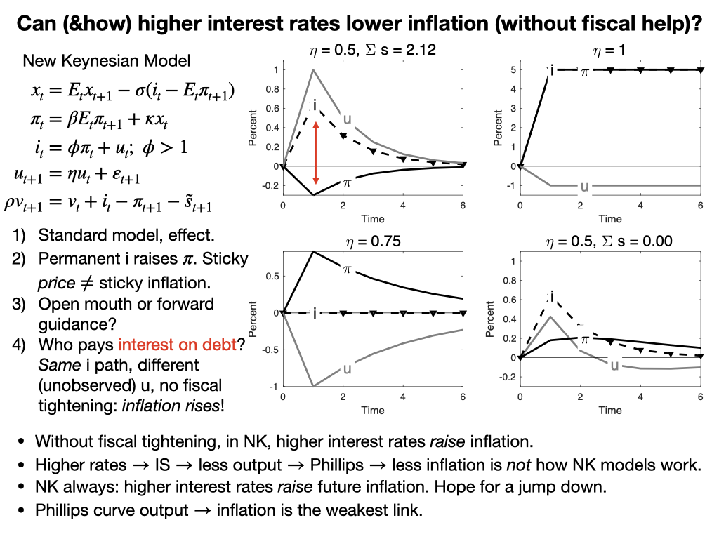
The equations are the utterly standard new-Keynesian model. The last equation tracks the evolution of the real value of the debt, which is usually in the footnotes of that model. 

OK, top right, the standard result. There is a positive but temporary shock to the monetary policy rule, u. Interest rates go up and then slowly revert. Inflation goes down. Hooray. (Output also goes down, as the Phillips Curve insists.) 

The next graph should give you pause on just how you interpreted the first one. What if the interest rate goes up persistently? Inflation rises, suddenly and completely matching the rise in interest rate! Yet prices are quite sticky -- k = 0.1 here. Here I drove the persistence all the way to 1, but that's not crucial. With any persistence above 0.75, higher interest rates give rise to higher inflation. 

What's going on? Prices are sticky, but inflation is not sticky. In the Calvo model only a few firms can change price in any instant, but they change by a large amount, so the rate of inflation can jump up instantly just as it does. I think a lot of intuition wants inflation to be sticky, so that inflation can slowly pick up after a shock. That's how it seems to work in the world, but sticky prices do not deliver that result. Hence, the real interest rate doesn't change at all in response to this persistent rise in nominal interest rates.  Now maybe inflation is sticky, costs apply to the derivative not the level, but absolutely none of the immense literature on price stickiness considers that possibility or how in the world it might be true, at least as far as I know. Let me know if I'm wrong. At a minimum, I hope I have started to undermine your faith that we all have easy textbook models in which higher interest rates reliably lower inflation. 

(Yes, the shock is negative. Look at the Taylor rule. This happens a lot in these models, another reason you might worry. The shock can go in a different direction from observed interest rates.) 

Panel 3 lowers the persistence of the shock to a cleverly chosen 0.75. Now (with sigma=1, kappa=0.1, phi= 1.2), inflation now moves with no change in interest rate at all.  The Fed merely announces the shock and inflation jumps all on its own. I call this "equilibrium selection policy" or "open mouth policy." You can regard this as a feature or a bug. If you believe this model, the Fed can move inflation just by making speeches! You can regard this as powerful "forward guidance." Or you can regard it as nuts. In any case, if you thought that the Fed's mechanism for lowering inflation is to raise nominal interest rates, inflation is sticky, real rates rise, output falls and inflation falls, well here is another case in which the standard model says something else entirely. 

Panel 4 is of course my main hobby horse these days. I tee up the question in Panel 1 with the red line. In that panel, the nominal interest are is higher than the expected inflation rate. The real interest rate is positive. The costs of servicing the debt have risen. That's a serious effect nowadays. With 100% debt/GDP each 1% higher real rate is 1% of GDP more deficit, $250 billion dollars per year. Somebody has to pay that sooner or later. This "monetary policy" comes with a fiscal tightening. You'll see that in the footnotes of good new-Keynesian models: lump sum taxes come along to pay higher interest costs on the debt. 

Now imagine Jay Powell comes knocking to Congress in the middle of a knock-down drag-out fight over spending and the debt limit, and says "oh, we're going to raise rates 4 percentage points. We need you to raise taxes or cut spending by $1 trillion to pay those extra interest costs on the debt." A laugh might be the polite answer. 

So, in the last graph, I ask, what happens if the Fed raises interest rates and fiscal policy refuses to raise taxes or cut spending? In the new-Keynesian model there is not a 1-1 mapping between the shock (u) process and interest rates. Many different u produce the same i. So, I ask the model, "choose a u process that produces exactly the same interest rate as in the top left panel,  but needs no additional fiscal surpluses." Declines in interest costs of the debt (inflation above interest rates) and devaluation of debt by period 1 inflation must match rises in interest costs on the debt (inflation below interest rates). The bottom right panel gives the answer to this question. 

Review: Same interest rate, no fiscal help? Inflation rises. In this very standard new-Keynesian model,  higher interest rates without a concurrent fiscal tightening raise inflation, immediately and persistently. 

Fans will know of the long-term debt extension that solves this problem, and I've plugged that solution before (see the "Expectations" paper above).

The point today: The statement that we have easy simple well understood textbook models, that capture the standard intuition -- higher nominal rates with sticky prices mean higher real rates, those lower output and lower inflation -- is simply not true. The standard model behaves very differently than you think it does. It's amazing how after 30 years of playing with these simple equations, verbal intuition and the equations remain so far apart. 

The last two bullet points emphasize two other aspects of the intuition vs model separation. Notice that even in the top left graph, higher interest rates (and lower output) come with rising inflation. At best the higher rate causes a sudden jump down in inflation -- prices, not inflation, are sticky even in the top left graph -- but then inflation steadily rises. Not even in the top left graph do higher rates send future inflation lower than current inflation. Widespread intuition goes the other way. 

In all this theorizing, the Phillips Curve strikes me as the weak link. The Fed and common intuition make the Phillips Curve causal: higher rates cause lower output cause lower inflation. The original Phillips Curve was just a correlation, and Lucas 1972 thought of causality the other way: higher inflation fools people temporarily to producing more. 

 

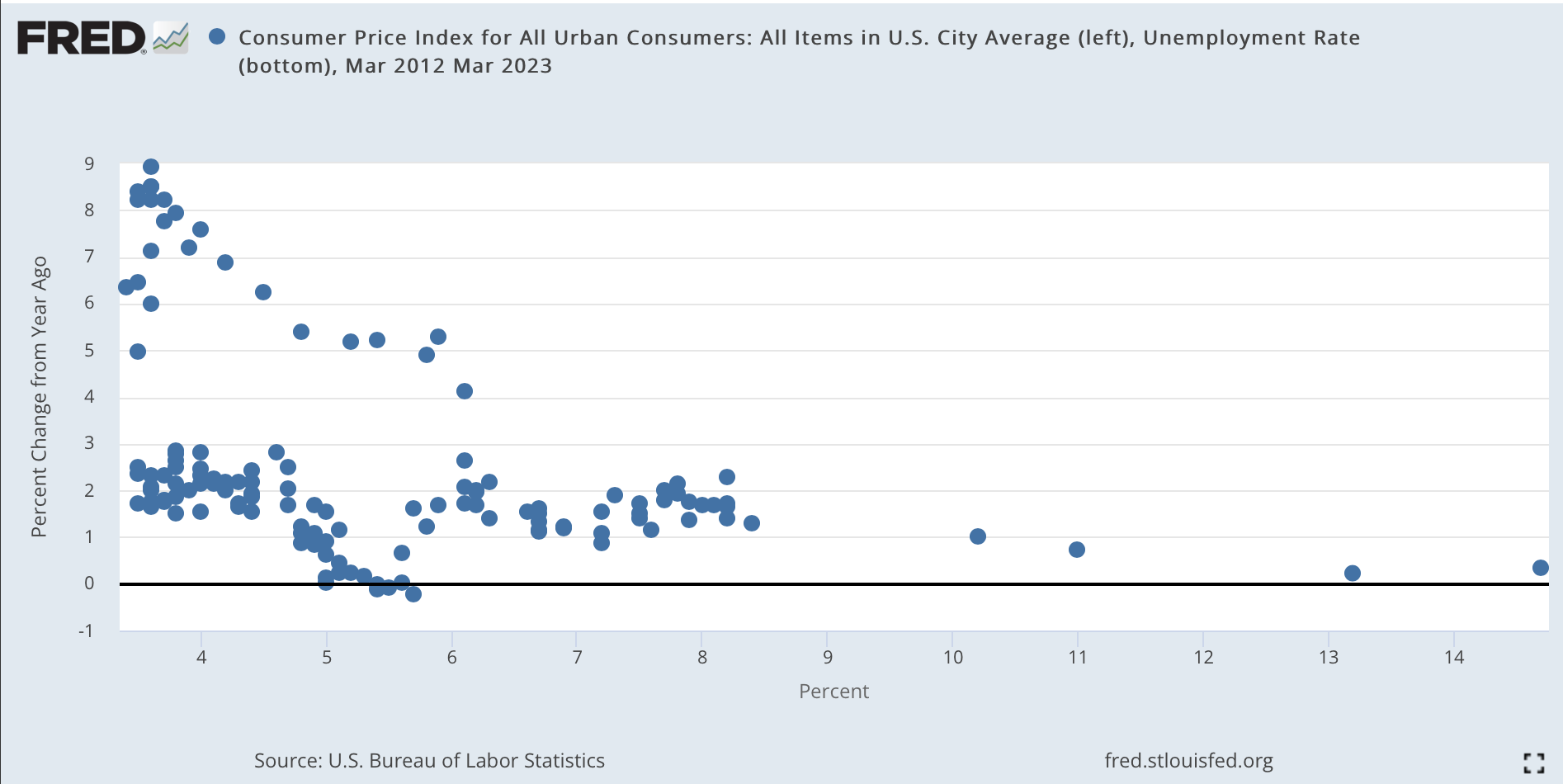
Here is the Phillips curve (unemployment x axis, inflation y axis) from 2012 through last month. The dots on the lower branch are the pre-covid curve, "flat" as common wisdom proclaimed. Inflation was still 2% with unemployment 3.5% on the eve of the pandemic. The upper branch is the more recent experience. 

I think this plot makes some sense of the Fed's colossal failure to see inflation coming, or to perceive it once the dragon was inside the outer wall and breathing fire at the inner gate. If you believe in a Phillips Curve, causal from unemployment (or "labor market conditions") to inflation, and you last saw 3.5% unemployment with 2% inflation in February 2021, the 6% unemployment of March 2021 is going to make you totally ignore any inflation blips that come along. Surely, until we get well past 3.5% unemployment again, there's nothing to worry about. Well, that was wrong. The curve "shifted" if there is a curve at all. 

But what to put in its place? Good question. 

Update:

Lots of commenters and correspondents want other Phillips Curves. I've been influenced by a number of papers, especially "New Pricing Models, Same Old Phillips Curves?" by Adrien Auclert, Rodolfo Rigato, Matthew Rognlie, and Ludwig Straub, and "Price Rigidity: Microeconomic Evidence and Macroeconomic Implications" by Emi Nakamura and  Jón Steinsson, that lots of different micro foundations all end up looking about the same. Both are great papers. Adding lags seems easy, but it's not that simple unless you overturn the forward looking eigenvalues of the system; "Expectations and the neutrality of interest rates" goes on in that way. Adding a lag without changing the system eigenvalue doesn't work. 

How many banks are in danger?

With amazing speed and impeccable timing, Erica Jiang, Gregor Matvos, Tomasz Piskorski, and Amit Seru analyze how exposed the rest of the banking system is to an interest rate rise.

Recap: SVB failed, basically, because it funded a portfolio of long-term bonds and loans with run-prone uninsured deposits. Interest rates rose, the market value of the assets fell below the value of the deposits. When people wanted their money back, the bank would have to sell at low prices, and there would not be enough for everyone. Depositors ran to be the first to get their money out. In my previous post, I expressed astonishment that the immense bank regulatory apparatus did not notice this huge and elementary risk. It takes putting 2+2 together: lots of uninsured deposits, big interest rate risk exposure. But 2+2=4 is not advanced math. 

How widespread is this issue? And how widespread is the regulatory failure? One would think, as you put on the parachute before jumping out of a plane,  that the Fed would have checked that raising interest rates to combat inflation would not tank lots of banks. 

Banks are allowed to report the "hold to maturity" "book value" or face value of long term assets. If a bank bought a bond for $100 (book value) or if a bond promises $100 in 10 years (hold to maturity value), basically, the bank may say it's worth $100, even though the bank might only be able to sell the bond for $75 if they need to stop a run. So one way to put the issue is, how much lower are mark to market values than book values? 

The paper (abstract):  

The U.S. banking system’s market value of assets is $2 trillion lower than suggested by their book value of assets accounting for loan portfolios held to maturity. Marked-to-market bank assets have declined by an average of 10% across all the banks, with the bottom 5th percentile experiencing a decline of 20%. 

... 10 percent of banks have larger unrecognized losses than those at SVB. Nor was SVB the worst capitalized bank, with 10 percent of banks have lower capitalization than SVB. On the other hand, SVB had a disproportional share of uninsured funding: only 1 percent of banks had higher uninsured leverage. 

... Even if only half of uninsured depositors decide to withdraw, almost 190 banks are at a potential risk of impairment to insured depositors, with potentially $300 billion of insured deposits at risk. ... these calculations suggests that recent declines in bank asset values very significantly increased the fragility of the US banking system to uninsured depositor runs.

Data:

we use bank call report data capturing asset and liability composition of all US banks (over 4800 institutions) combined with market-level prices of long-duration assets. 

How big and widespread are unrecognized losses?

The average banks’ unrealized losses are around 10% after marking to market. The 5% of banks with worst unrealized losses experience asset declines of about 20%. We note that these losses amount to a stunning 96% of the pre-tightening aggregate bank capitalization.

Percentage of asset value decline when assets are mark-to- market according to market price growth from 2022Q1 to 2023Q1

Most banks operate with (to my mind) tiny slivers of capital -- 10% or less. So 10% decline in asset value is a lot! (Banks get money by issuing stock and borrowing. The capitalization ratio is how much money banks get by issuing stock/assets. Capital is not reserves, liquid assets "held" to satisfy depositors.) In the right panel, the problem is not confined to small banks and small amounts of dollars. 

But...all of this is slightly old data. How much worse will this get if the Fed raises interest rates a few more percentage points? A lot. 

To runs, it takes 2+2 to get 4. How widespread is reliance on uninsured, run-prone deposits? (Or, deposits that were run-prone until the Fed and Treasury ex-post guaranteed all deposits!) Here SVB was an outlier. 

The median bank funds 9% of their assets with equity, 65% with insured deposits, and 26% with uninsured debt comprising uninsured deposits and other debt funding....SVB did stand out from other banks in its distribution of uninsured leverage, the ratio of uninsured debt to assets...SVB was in the 1st percentile of distribution in insured leverage. Over 78 percent of its assets was funded by uninsured deposits.

But it is not totally alone 

the 95th percentile [most dangerous] bank uses 52 percent of uninsured debt. For this bank, even if only half of uninsured depositors panic, this leads to a withdrawal of one quarter of total marked to market value of the bank. 

Uninsured deposit to asset ratios calculated based on 2022Q1 balance sheets and mark-to-market values 

Overall, though, 

...we consider whether the assets in the U.S. banking system are large enough to cover all uninsured deposits. Intuitively, this situation would arise if all uninsured deposits were to run, and the FDIC did not close the bank prior to the run ending. ...virtually all banks (barring two) have enough assets to cover their uninsured deposit obligations. ... there is little reason for uninsured depositors to run.

... SVB, is [was] one of the worst banks in this regard. Its marked-to-market assets are [were] barely enough to cover its uninsured deposits.

Breathe a temporary sigh of relief. 

I am struck in the tables by the absence of wholesale funding. Banks used to get a lot of their money from repurchase agreements, commercial paper, and other uninsured and run-prone sources of funding. If that's over, so much the better. But I may be misunderstanding the tables. 

Summary: Banks were borrowing short and lending long, and not hedging their interest rate risk. As interest rates rise, bank asset values will fall. That has all sorts of ramifications. But for the moment, there is not a danger of a massive run. And the blanket guarantee on all deposits rules that out anyway. 

Their bottom line: 

There are several medium-run regulatory responses one can consider to an uninsured deposit crisis. One is to expand even more complex banking regulation on how banks account for mark to market losses. However, such rules and regulation, implemented by myriad of regulators with overlapping jurisdictions might not address the core issue at hand consistently 

I love understated prose.

There does need to be retrospective. How are 100,000 pages of rules not enough to spot plain-vanilla duration risk -- no complex derivatives here -- combined with uninsured deposits? If four authors can do this in a weekend, how does the whole Fed and state regulators miss this in a year? (Ok, four really smart and hardworking authors, but still... ) 

Alternatively, banks could face stricter capital requirement... Discussions of this nature remind us of the heated debate that occurredafter the 2007 financial crisis, which many might argue did not result in sufficient progress on bank capital requirements...

My bottom line (again) 

This debacle goes to prove that the whole architecture is hopeless: guarantee depositors and other creditors, regulators will make sure that banks don't take too many risks. If they can't see this, patching the ship again will not work. 

If banks channeled all deposits into interest-paying reserves or short-term treasury debt, and financed all long-term lending with long-term liabilities, maturity-matched long-term debt and lots of equity, we would end private sector financial crises forever. Are the benefits of the current system worth it? (Plug for "towards a run-free financial system." "Private sector" because a sovereign debt crisis is something else entirely.) 

(A few other issues stand out in the SVB debacle. Apparently SVB did try to issue equity, but the run broke out before they could do so. Apparently, the Fed tried to find a buyer, but the anti-merger sentiments of the administration plus bad memories of how buyers were treated after 2008 stopped that. Beating up on mergers and buyers of bad banks has come back to haunt our regulators.) 

Update: 

(Thanks to Jonathan Parker) It looks like the methodology does not mark to market derivatives positions. (It would be hard to see how it could do so!) Thus a bank that protects itself with swap contracts would look worse than it actually is. (Translation: Banks can enter a contract that costs nothing, in which they pay a fixed rate of interest and receive a floating rate of interest. When interest rates go up, this contract makes a lot of money! )

Amit confirms,

As we say in our note, due to data limitations, we do not account for interest rate hedges across the banks. As far as we know SVB was not using such hedges...

Of course if they are, one has to ask who is the counterparty to such hedges and be sure they won't similarly blow up. AIG comes to mind. 

He adds: 

note we don’t account for changes in credit risk on the asset side. All things equal this can make things worse for borrowers and their creditors with increases in interest rates. Think for a moment about real estate borrowers and pressures in sectors such as commercial real estate/offices etc. One could argue this number would be large.  

So don't sleep too well.  

From an email correspondent: 

Besides regulation, accountancy itself is a joke. KPMG Gave SVB, Signature Bank Clean Bill of Health Weeks Before Collapse.  

How can unrealised losses near equal to a bank's capital be ignored in the true and fair assessment of its financial condition (the core statement of an audit leaving out all the disclaimers) just because it was classified as Held to Maturity owing some nebulous past "intention" (whatever that was ever worth) not to sell?

It strikes me that both accounting and regulation have become so complicated that they blind intelligent people to obvious elephants in the room.  

Lessons from Sargent and Leeper

At the AEI fiscal theory event last Tuesday Tom Sargent and Eric Leeper made some key points about the current situation, with reference to lessons of history. 

Tom's comments updated his excellent paper with George Hall "Three World Wars" (at pnas,  summary essay in the Hoover Conference volume). Tom and George liken covid to a war: a large emergency requiring immense expenditure. We can quibble about "require" but not the expenditure. 

(2008 was a little war in this sense as well.) Since outlays are well ahead of receipts, these huge temporary expenditures are financed by issuing debt and printing money, as optimal tax theory says they should be. 

In all three cases, you see a ratcheting up of outlays after the war. That's happening now, and in 2008, just as in WWI and WWII. 

After WWI and WWII, there is a period of primary surpluses -- tax receipts greater than spending -- which helps to pay back the debt. This time is notable for the absence of that effect. 

We see that most clearly by plotting the primary deficits directly. The data update since Tom and George's original paper (dots) makes that clear. To a fiscal theorist, this is a worrisome difference. We are not following historical tradition of regular, full employment, peacetime surpluses. 

The two world wars were also financed by a considerable inflation. The important consequence of inflation is that it inflates away government debt. Essentially, we pay for part of the war by a default on debt, engineered via inflation. 

1947 is an interesting case. As now, inflation broke out, the Fed left interest rates alone, and the inflation went away once it had inflated away enough debt. That too is an interesting episode in the debate whether the Fed must move rates more than one for one to keep inflation from spiraling away. 

The effect of inflation is clearer in the next graph, which plots the real return on government bonds: 

Yes, the inflation of 1920 did inflate away a lot of the WWI debt, though the deflation of 1921 brought a lot of that back. (This is an episode we would do well to remember more! The price level doubled from 1916 through 1920. It then retreated by a third in 1920-1921. There was a sharp recession, but the economy recovered very quickly with no stimulus or heroic measures. The conventional wisdom that wringing out WWI inflation caused the UK 1920s doldrums needs to consider this counterexample. But back to our point) 

This is also consistent with standard optimal tax theory, which says that in the event of a disaster that happens once every 50 years or so, it is right to execute a "state contingent default" (Lucas and Stokey), and inflation is a natural way to do it. 

But... "state contingent default" is supposed to happen at the beginning of a war. These inflations happened at the end of the war. How did governments sell bonds to people who should have expected them to be inflated away? Yes, there were some price controls and financial repression, but it's still an important puzzle to standard public finance theory.  

My concern, of course, is that we've had two once in a hundred year events in a row (2008, 2020), I can think of lots more that might come soon, and you can only do this occasionally. Hit people over the head a few too many times and they start to duck. We will head to the next crisis with no history of steady surpluses in good times, 100% debt to GDP ratio, and a painful reminder of what happens if you lend to the US right in the rear view mirror. 

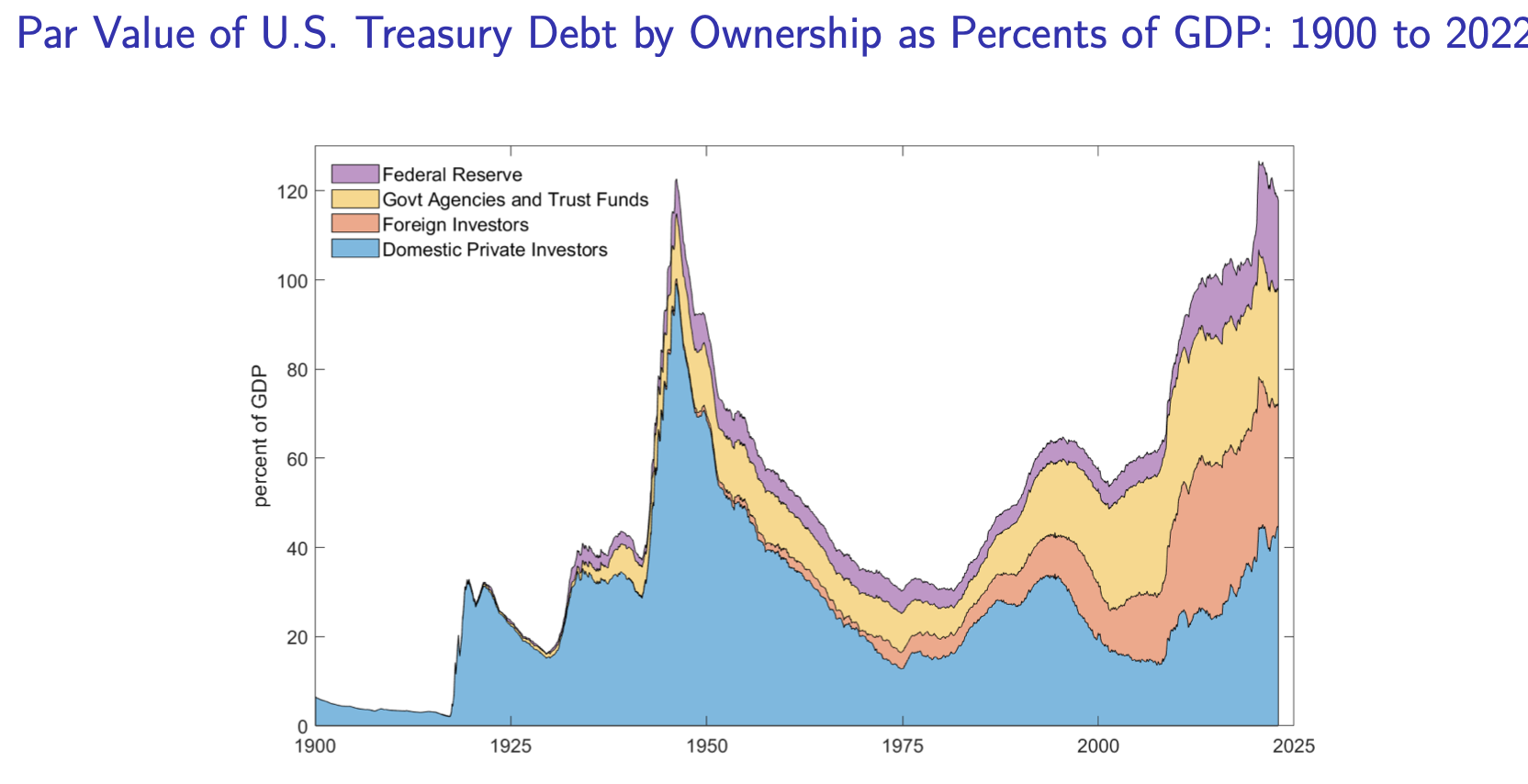
We start the H5N1/Taiwan war crisis with the same debt we had at the end of WWII. And who owns the debt leads to some fascinating speculation which I'll let you fill in with your chat GPT.  

Tom closed by echoing my favorite bright idea for avoiding the debt limit: Since the limit applies to par value not market value, the Treasury can issue all the perpetuities it wants. That's far better than the trillion dollar coin, though I suspect the Supreme Court would take just as dim a view of it. 

Eric  brought up a great point from his super Recovery of 1933 paper with Margaret Jacobson and Bruce Preston. 

In 1933, we had a disastrous deflation. The gold standard is a lovely fiscal commitment device to try to contain inflation, but it has an Achilles heel. If there is a deflation, the government has to raise taxes to pay an unexpected real windfall to bondholders. In 1933, the Roosevelt Administration abrogated the gold standard. It was a default on the legal terms of the bonds. And look what happened to inflation! 

Eric also brought up a second central point of his 1933 paper: The Roosevelt Administration separated the budget into a "regular" budget, in which we should expect deficits to be paid back, and an "emergency" budget, unbacked (in our language) by expected surpluses. That cleverly allowed inflationary finance in 1933, but once the "emergency" was over in 1941, it preserved the US reputation for repaying wartime debts with subsequent surpluses, and allowed it to borrow for WWII. This loss of "back to normal," of expectations that we are now in "regular" not "emergency" finance is worrisome today. 

Finally, Eric brought some nice evidence to bear on the question, why 2020 but not 2008? Well, in part, we can look at statements of public officials. In 2008, they explicitly said, deficit now, repayment later. In 2020 they explicitly said the opposite. 

("Offsets" is Washington-speak for "taxes" or later spending cuts.) Don't read a pejorative in this analysis. If you want to borrow, finance crisis expenditures and not create inflation, you "maintain the norm." If you want to create a "state contingent default" and pay for crisis expenditures by inflating away debt, you have to "violate the norm." That is darn hard -- ask the Japanese. How do you convince people you're not going to repay some part of the debt, despite a good reputation, but just some part, and if WWII comes along you're good for additional debts? Well, announcing your intentions helps!  

And it worked. We very quickly inflated away the debt. Creating a state contingent default via inflation is not easy. Still to be seen though is whether we can return to "normal" "Hamilton norm" once it's over. 

Robert Barro also had great comments, but more directed at the book and with no great graphs to pass along. Thanks anyway!