I just finished a new draft of "Expectations and the neutrality of interest rates," which includes some ruminations on inflation that may be of interest to blog readers.
A central point of the paper is to ask whether and how higher interest rates lower inflation, without a change in fiscal policy. That's intellectually interesting, answering what the Fed can do on its own. It's also a relevant policy question. If the Fed raises rates, that raises interest costs on the debt. What if Congress refuses to tighten to pay those higher interest costs? Well, to avoid a transversality condition violation (debt that grows forever) we get more inflation, to devalue outstanding debt. That's a hard nut to avoid.
But my point today is some intuition questions that come along the way. An implicit point: The math of today's macro is actually pretty easy. Telling the story behind the math, interpreting the math, making it useful for policy, is much harder.
1. The Phillips curve
The Phillips curve is central to how the Fed and most policy analysts think about inflation. In words, inflation is related to expected future inflation and by some measure if economic tightness, factor \(x\). In equations, \[ \pi_t = E_t \pi_{t+1} + \kappa x_t.\] Here \(x_t\) represents the output gap (how much output is above or below potential output), measures of labor market tightness like unemployment (with a negative sign), or labor costs. (Fed Governor Chris Waller has a great speech on the Phillips curve, with a nice short clear explanation. There are lots of academic explanations of course, but this is how a sharp sitting member of the FOMC thinks, which is what we want to understand. BTW, Waller gave an even better speech on climate and the Fed. Go Chris!)
So how does the Fed change inflation? In most analysis, the Fed raises interest rates; higher interest rates cool down the economy lowering factor x; that pushes inflation down. But does the equation really say that?
This intuition thinks of the Phillips curve as a causal relation, from right to left. Lower \(x\) causes lower inflation. That's not so obvious. In one story, the Phillips curve represents how firms set prices, given their expectation of other's prices and costs. But in another story, aggregate demand raises prices, and that causes firms to hire more (Chris Waller emphasized these stories).
This reading may help to digest an otherwise puzzling question: Why are the Fed and its watchers so obsessed with labor markets? This inflation certainly didn't start in labor markets, so why put so much weight on causing a bit of labor market slack? Well, if you read the Phillips curve from right to left, that looks like the one lever you have. Still, since inflation clearly came from left to right, we still should put more emphasis in curing it that way.
2. Adjustment to equilibrium vs. equilibrium dynamics.
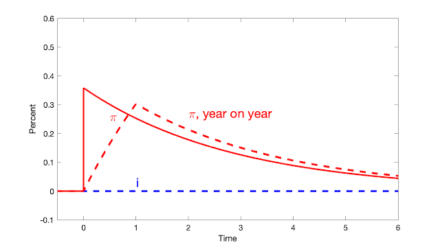
But does the story work? Lower \(x_t\) lowers inflation \(\pi_t\) relative to expected future inflation \(E_t \pi_{t+1}\). Thus, it describes inflation that is rising over time. This does not seem at all what the intuition wants.
So how do we get to the intuition that lower \(x_t\) leads to inflation got goes down over time? (This is on p. 16 of the paper by the way.) An obvious answer is adaptive expectations: \(E_t \pi_{t+1} = \pi_{t-1}\). Then lower \(x_t\) does mean inflation today lower than it was in the past. But the Fed and most commenters really don't want to go there. Expectations may not be "rational," and in most commentary they are either "anchored" by faith in the Fed, or driven by some third force. But they aren't mechanically last year's inflation. If they were, we would need much higher interest rates to get real interest rates above zero. Perhaps the intuition comes from remembering these adaptive expectations dynamics, and not realizing that the new view that expectations are forward looking, even if not rational, undermines those dynamics.
Another answer may be confusion between adjustment to equilibrium and movement of equilibrium inflation over time. Lower \(x_t\) means lower inflation \(\pi_t\) than would otherwise be the case. But that reduction is an adjustment to equilibrium. It's not how inflation we observe -- by definition, equilibrium inflation -- evolves over time.
This is, I think, a common confusion. It's not always wrong. In some cases, adjustment to equilibrium does describe how an equilibrium quantity changes, and in a more complex model that adjustment plays out as a movement over time. For example, a preference or technology shock might give a sudden increase in capital; add adjustment costs and capital increases slowly over time. A fiscal shock or money supply shock gives a sudden increase in the price level; add sticky prices and you get a slow increase in the price level over time.
But we already have sticky prices. This is supposed to be the model, the dynamic model, not a simplified model. Here, inflation lower than it otherwise would be is not the same thing as inflation that goes down slowly over time. It's just a misreading of equations.
Another possibility is that verbal intuition refers to the future, \[ E_t \pi_{t+1} = E_t \pi_{t+2} + \kappa E_t x_{t+1} .\]Now, perhaps, raising interest rates today lowers future factor x, which then lowers future inflation \(E_t\pi_{t+1}\) relative to today's inflation \(\pi_t\). That's still a stretch however. First, the standard new-keynesian model does not have such a delay. \[x_t = E_t x_{t+1} - \sigma(i_t - E_t \pi_{t+1})\]says that higher interest rates also immediately lower output, and lower output relative to future output. Higher interest rates also raise output growth. This one is more amenable to adding frictions -- habits, capital accumulation, and so forth -- but the benchmark model not only does not have long and variable lags, it doesn't have any lags at all. Second, maybe we lower inflation \(\pi_{t+1}\) relative to its value \(\pi_t\), in equilibrium, but we still have inflation growing from \(t+1\) to \( t+2\). We do not have inflation gently declining over time, which the intuition wants.
We are left -- and this is some of the point of my paper -- with a quandary. Where is a model in which higher interest rates lead to inflation that goes down over time? (And, reiterating the point of the paper, without implicitly assuming that fiscal policy comes to the rescue.)
3. Fisherian intuition
A famous economist, who thinks largely in the ISLM tradition, once asked me to explain in simple terms just how higher interest rates might raise inflation. Strip away all price stickiness to make it simple, still, the Fed raises interest rates and... now what? Sure point to the equation \( i_t = r + E_t\pi_{t+1} \) but what's the story? How would you explain this to an undergraduate or MBA class? I fumbled a bit, and it took me a good week or so to come up with the answer. From p. 15 of the paper,
First, consider the full consumer first-order condition \[x_t = E_t x_{t+1} - \sigma(i_t -E_t \pi_{t+1})\] with no pricing frictions. Raise the nominal interest rate \(i_t\). Before prices change, a higher nominal interest rate is a higher real rate, and induces people to demand less today \(x_t\) and more next period \(x_{t+1}\). That change in demand pushes down the price level today \(p_t\) and hence current inflation \(\pi_t = p_t - p_{t-1}\), and it pushes up the expected price level next period \(p_{t+1}\) and thus expected future inflation \(\pi_{t+1}=p_{t+1}-p_t\).
So, standard intuition is correct, and refers to a force that can lower current inflation. Fisherian intuition is correct too, and refers to a natural force that can raise expected future inflation.
But which is it, lower \(p_t\) or higher \(p_{t+1}\)? This consumer first-order condition, capturing an intertemporal substitution effect, cannot tell us. Unexpected inflation and the overall price level is determined by a wealth effect. If we pair the higher interest rate with no change in surpluses, and thus no wealth effect, then the initial price level \(p_t\) does not change [there is no devaluation of outstanding debt] and the entire effect of higher interest rates is a rise in \(p_{t+1}\). A concurrent rise in expected surpluses leads to a lower price level \(p_t\) and less current inflation \(\pi_t\). Thus in this context standard intuition also implicitly assumes that fiscal policy acts in concert with monetary policy.
In both these stories, notice how much intuition depends on describing how equilibrium forms. It's not rigorous. Walrasian equilibrium is just that, and does not come with a price adjustment process. It's a fixed point, the prices that clear markets, period. But believing and understanding how a model works needs some sort of equilibrium formation story.
4. Adaptive vs. rational expectations
The distinction between rational, or at least forward-looking and adaptive or backward-looking expectations is central to how the economy behaves. That's a central point of the paper. It would seem easy to test, but I realize it's not.
Writing in May 2022, I thought about adaptive (backward-looking) and rational (forward-looking), and among other points that under adaptive expectations we need nominal interest rates above current inflation -- i.e. much higher -- to imply real interest rates, while that isn't necessarily true with forward-looking expectations. You might be tempted to test for rational expectations, or look at surveys to pronounce them "rational" vs. "behavioral," a constant temptation. I realize now it's not so easy (p. 44):
Expectations may seem adaptive. Expectations must always be, in equilibrium, functions of variables that people observe, and likely weighted to past inflation. The point of "rational expectations'' is that those forecasting rules are likely to change as soon as a policy maker changes policy rules, as Lucas famously pointed out in his "Critique." Adaptive expectations may even be model-consistent [expectations of the model equal expectations in the model] until you change the model.
That observation is important in the current policy debate. The proposition that interest rates must be higher than current inflation in order to lower inflation assumes that expected inflation equals current inflation -- the simple one-period lagged adaptive expectations that I have specified here. Through 2021-2022, market and survey expectations were much lower than current (year on year) inflation. Perhaps that means that markets and surveys have rational expectations: Output is temporarily higher than the somewhat reduced post-pandemic potential, so inflation is higher than expected future inflation (\(\pi_t = E_t \pi_{t+1} + \kappa x_t\)). But that observation could also mean that inflation expectations are a long slow-moving average of lagged inflation, just as Friedman speculated in 1968 (\(\pi^e_t = \sum_{j=1}^\infty \alpha_j \pi_{t-j}\)). In either case, expected inflation is much lower than current inflation, and interest rates only need to be higher than that low expectation to reduce inflation. Tests are hard, and you can't just look at in-sample expectations to proclaim them rational or not.
5. A few final Phillips curve potshots
It is still a bit weird that so much commentary is so focused on the labor market to judge pressure on inflation. This inflation did not come from the labor market!
Some of this labor market focus makes sense in the new-Keynesian interpretation of the Phillips curve: Firms set prices based on expected future prices of their competitors and marginal costs, which are largely labor costs. That echoes the 1960s "cost push" view of inflation (as opposed to its nemesis "demand pull" inflation). But it begs the question, well, why are labor costs going up? The link from interest rates to wages is about as direct as the link from interest rates to pries. This inflation did not come from labor costs, maybe we should fix the actual problem? Put another way, the Phillips curve is not a model. It is part of a model, and lots of equations have inflation in them. Maybe our focus should be elsewhere.
Back to Chris Waller, whose speech seems to me to capture well sophisticated thinking at the Fed. Waller points out how unreliable the Phillips curve is
What do economic data tell us about this relationship? We all know that if you simply plot inflation against the unemployment rate over the past 50 years, you get a blob. There does not appear to be any statistically significant correlation between the two series.

In more recent years, since unemployment went up and down but inflation didn't go far, the Phillips curve seemed "flat,"
the Phillips curve was very flat for the 20-plus years before the pandemic,
You can see this in the decline of unemployment through 2020, as marked, with no change in inflation. Then, unemployment surged in 2021, again with no deflation. 2009 was the last time there was any slope at all to the Phillips curve.
But is it "flat" -- a stable, exploitable, flat relationship -- or is it just a stretched out "blob", two series with no stable relationship, one of which just got stable?
In any case, as unemployment went back down to 3.5 percent in 2022, inflation surged. You can forgive the Fed a bit: We had 3.5% unemployment with no inflation in 2020, why should we worry about 3.5% unemployment in 2022? I think the answer is, because inflation is driven by a whole lot more than unemployment -- stop focusing on labor markets!
A flat curve, if it is a curve, is depressing news:
Based on the flatness of the Phillips curve in recent decades, some commentators argued that unemployment would have to rise dramatically to bring inflation back down to 2 percent.
At best, we retrace the curve back to 2021 unemployment. But (I'll keep harping on this), note the focus on the error-free Phillips curve as if it is the entire economic model.
Waller views the new Phillips curve as a "curve," that has become steeper, and cites confirming evidence that prices are changing more often and thus becoming more flexible.
... considering the data for 2021... the Phillips curve suddenly looked relatively steep.. since January 2022, the Phillips curve is essentially vertical: The unemployment rate has hovered around 3.6 percent, and inflation has varied from 7 percent (in June) to 5.3 percent (in December).
Waller concludes
A steep Phillips curve means inflation can be brought down quickly with relatively little pain in terms of higher unemployment. Recent data are consistent with this story.
Isn't that nice -- from horizontal to vertical all on its own, and in the latest data points inflation going straight down.
Still, perhaps the right answer is that this is still a cloud of coincidence and not the central, causal, structural relationship with which to think about how interest rates affect inflation.
If only I had a better model of inflation dynamics...


Tidak ada komentar:
Posting Komentar